In today's instalment of Tales from the Pixel Mines: Gradients and the binary tree texture! We'll also discuss the new Quantize and GradientMap filters.
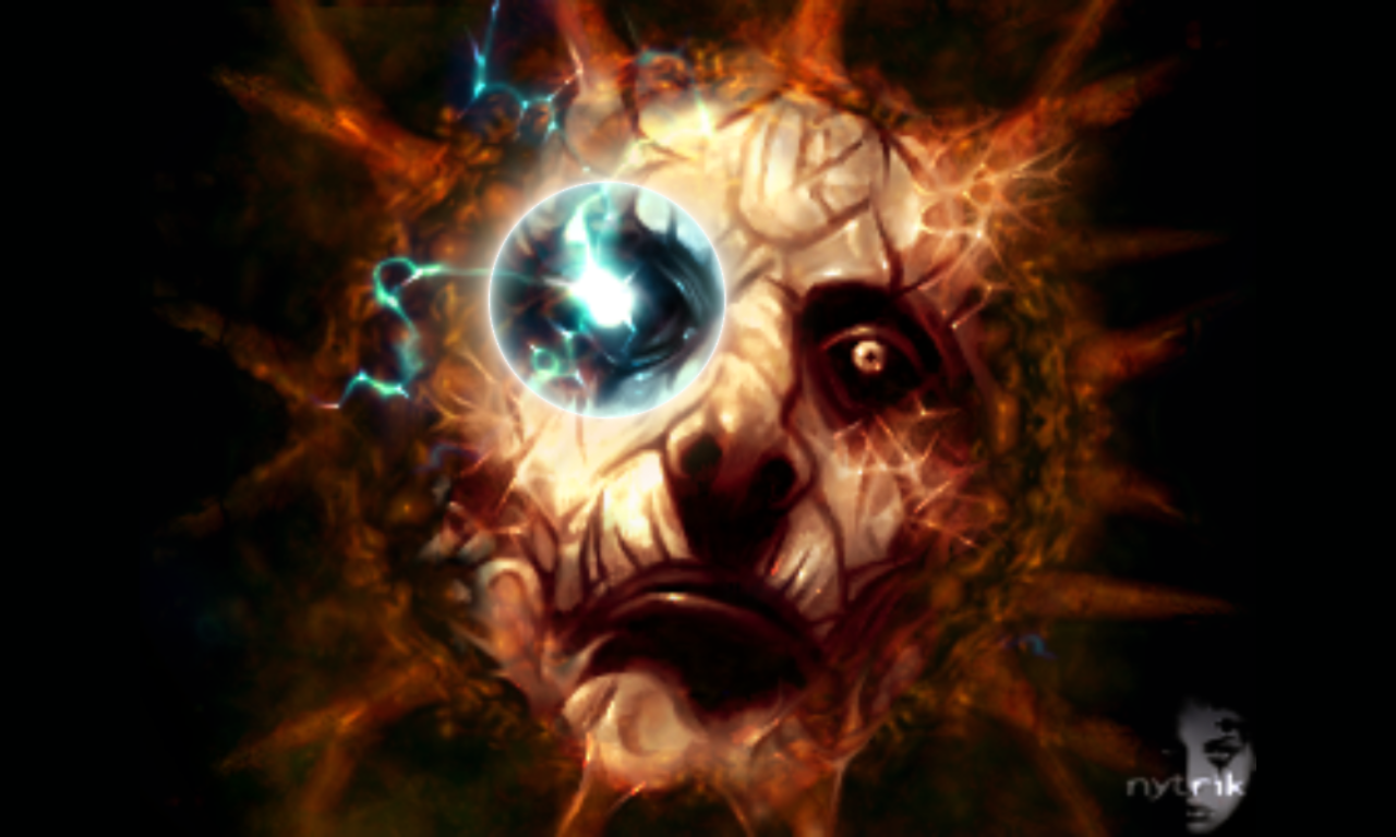 Pictured: a gradient used as a lens flare.
Phaser 3 Gradients
In Phaser 3, Gradient was an FX (the predecessor of Filters). It created a linear gradient from one color to another, between two points, overwriting the colors of another object. Optionally, the gradient would proceed in steps instead of making a smooth color.
This seemed limited. A gradient is more like a texture, not something you do to an object. And gradients can do a lot more than just a linear blend of RGB values.
Possibilities of Gradients
At its heart, a gradient is a way to map an input of 0-1 to some output color. The simplest version just blends a start and end color, but you can go much further.
You can divide up that range into smaller bands, each with its own color choices and interpolation settings. Those interpolations can vary how fast the interpolation proceeds, and the color space it occurs in. This is commonly seen in more advanced editing programs, sometimes as a predefined "fill pattern", sometimes as a gradient you can edit yourself. I took particular inspiration from ramps in Autodesk Maya, and custom gradients in The GIMP. This general approach seems to have worked for decades. Many editing programs don't offer this level of control, however.
The shape of the gradient is also an option. Editing programs do generally offer options for shape, even if it's something as simple as linear versus radial.
And I always wanted gradients to be flexible. There are many places where gradients can be used as the basis of other effects.
Phaser 4 Gradients
This all came together to inform the new Gradient in Phaser 4.
Gradient is now a Game Object, so it doesn't need to replace something else. It extends Shader, so it has all the Shader capabilities. In particular, setRenderToTexture() allows you to turn the object into a texture, which makes it accessible to the rest of the rendering system. As a Shader, it renders pixels, so it isn't limited to texel resolution: each pixel on the screen evaluates the shader precisely.
I implemented a flexible color ramp format. You can do a simple gradient just like before, or a crazy gradient with up to a million bands. You can use defaults, or configure the interpolation and color space for each band. I want to support simple and advanced approaches.
The gradient also supports a range of shapes: linear, bilinear, radial, and symmetric and asymmetric conic shapes.
Let's look at the details and some rendering secrets.
Color Bands
At the base of the gradient is a color band. This is just some part of the gradient range. It has a color at either end, and interpolation settings. This is stored in a ColorBand object.
The simplest band covers the whole gradient, and goes from black to white. Easy! But you have more options.
You can set colors, of course. The config options support several formats:
- Integers, e.g.
0xff00ff. This format supports alpha input, but it's a bit fiddly and I don't recommend it unless you know what you're doing. For example,0x00ffff00looks like it should be RGBA for transparent cyan, but it's actually the same as0xffff00because leading 0s are discarded. - Tuples, e.g.
[ 1, 0, 1, 0 ]. This is a better way to handle alpha input, because its position is clearly defined. - Strings, e.g.
#ff00ff. Phaser doesn't support alpha in string input. - A Phaser
Colorobject.
You can set the color space within the band.
- RGBA, blending color channels directly. This has a tendency to produce darker interpolations.
- HSVA_NEAREST, converting from RGB to hue, saturation, and value, then interpolating those values. This tends to produce brighter interpolation.
- HSVA_PLUS, working in HSV but always increasing the hue. For example, the blend from green to yellow would have to go through blue, purple, and red to wrap around.
- HSVA_MINUS, working in HSV but always decreasing the hue. Like PLUS, this is useful when you know you want a specific color transition.
You can set the middle of the band: default 0.5, range 0-1. This alters the base curve before interpolation.
You can set the interpolation within each band.
- LINEAR, the raw number.
- CURVED, changing rapidly at start and end, good for convex surfaces.
- SINUSOIDAL, changing rapidly at the middle, good as part of smooth transitions.
- CURVE_START, changing quickly at the start and flattening at the end.
- CURVE_END, changing quickly at the end and flattening at the start.
And you can set the start and end of the band, within the 0-1 range of the ramp. When creating bands as a ramp from configs, you can instead set a size, which appends to the end of the previous band, for convenience.
Note that bands don't have to share colors or modes. You can use the same color for end and start, to create a smooth transition, but you can set them completely different.
Color Ramps
A ColorRamp object stores a full range of color bands. It's mostly responsible for constructing color bands and the data formats used during rendering.
It also supports various queries and manipulations. You can sample the ramp without rendering it with getColor(index). You can split bands up with splitBand(). You can even tidy up messy ramps with fixFit().
ColorRamp is an essential part of Gradient, but you can also use it by itself.
Gradient Shapes and Repetition
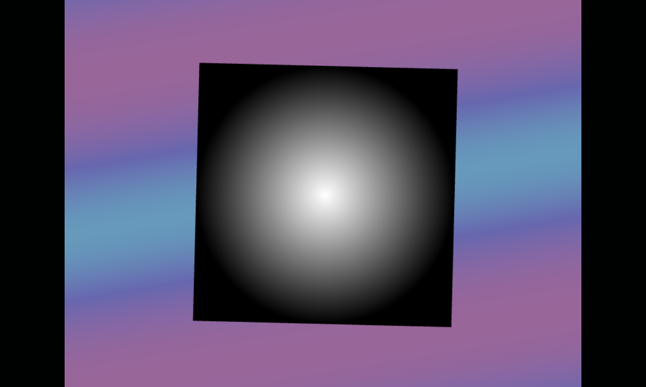
The gradient itself maps space to the ramp. This includes the actual shape, the shape mode, and the repeat mode.
The shape is defined by a start and a shape vector. You can instead define a length and direction for the shape vector. By default, the start is on the left, and the shape vector goes to the right side. For radial and conic gradients, you probably want to put the start in the middle, and reduce the length of the shape vector.
The shape mode offers linear, bilinear, radial, and symmetric and asymmetric conic gradients. These change the 2D coordinate on the gradient quad into the 1D value for the ramp. This can produce ramp values outside the range 0-1, in combination with the shape start/vector. For example, a radial gradient with length 0.5 and a start in the middle will reach a ramp value of 1 at the middle of the edges, and about 1.4 at the corners of the quad.
The repeat mode maps the ramp value from its raw value to the 0-1 range. The following functions are available:
- EXTEND: The colors at both ends of the ramp continue. Radial and conic gradients don't have anything below 0. Note that the ends aren't necessarily at 0 and 1, although it is more logical to set it up that way, and values below 0 and above 1 will probably never be seen. (The opening image of this article only has bands for a small part of the ramp!)
- TRUNCATE: Anything outside the range 0-1 is transparent.
- SAWTOOTH: The gradient repeats over and over. This can be a sharp transition, but if you line up the start and end using multiple bands, you can make it smooth.
- TRIANGULAR: The gradient goes back and forth from 0 to 1 and back. This is naturally smooth.
You can see examples of all these at labs.phaser.io.
Rendering Secrets: Binary Trees and Dithering in Phaser 4
Now for the deeply technical stuff.
Gradients include two pretty sophisticated pieces of technology: a data texture for encoding color ramps, and interleaved gradient noise for dithering.
Data Texture Encoding
The ColorRamp object contains the data for the Gradient shader to render an actual gradient. Unfortunately, the shader can only accept a fairly small amount of data as shader uniforms. WebGL only requires a minimum of 64 uniforms available to a fragment shader. What do?
Well, we could choose to render the gradient as a series of strips. However, we have radial gradients, and these would quickly require vast numbers of triangles. And even linear gradients would use more triangles than a simple quad, if multiple color bands are included.
We could also just not render multiple color bands, and limit gradients to 2 colors. But I don't like that restriction.
So we encode the ColorRamp into a texture. We can sample that texture, and interpret its colors as numbers. But that has its challenges, too. We can't just encode pairs of colors and the band data, because for a given pixel, we don't know which pair it belongs to. We'd have to check them all - and for a complex gradient, that means a whole lot of samples. Very inefficient.
Instead, I added a binary tree to the start of the texture. This is a simple data structure, where each node has two child nodes. In this case, the nodes consist of the end position of each band. We split the bands down the middle, and put the central value first. Then we split each of those halves down the middle, and put that pair of central values next, and so on until every band has added its end position to the tree. To find the band corresponding to the current gradient position, we compare that value to the start of the tree, and then pick either the left or the right path by comparing the position to the end of the band. We walk down the nodes to the end, and we have the correct band.
Now, there are some caveats here. First, the tree must be symmetrical. If it doesn't have enough branches to completely populate the final level, weird stuff happens. So we pad it out. Second, it must have constant size at compile time. The GLSL shader language doesn't allow us to write loops with unpredictable length. We must compile the shader to a specific length. Fortunately, Phaser 4 supports shader variants, and symmetrical trees can only have a few sizes based on powers of 2. A gradient with a thousand bands is just level 9; the largest possible gradients (with a million bands, limited by the size of a 4096x4096 texture) don't go past level 20. In all probability, you're not going to need more than a handful of variants, and the maximum is just 20.
These numbers also demonstrate how efficient the binary tree is. Each choice splits the candidate list in half. Put another way, given n choices, we get 2^n options. So instead of checking a thousand bands, we can just check 10 nodes in the tree.
And that's how we can render a million bands in a single quad.
Interleaved Gradient Noise Dithering
What is dithering? Why is dithering?
Well, computers have limited precision. A modern display can handle 16 million colors, but it does it by combining three channels of just 256 colors each. That means there are not very many levels of brightness available. If we render a gradient naively, we will change the brightness level at the same rate across nearby pixels, and this leads to "banding": obvious lines of brightness changes, often seen in skies and bright glows.
Dithering is the process of introducing a deliberate error to mess with that clear, predictable pattern. There are many kinds of dithering. Floyd-Steinberg Error Diffusion is an excellent example; it tracks the difference between the output and the true value in a higher-precision format. This "error" is "diffused" onto nearby pixels that haven't been processed yet, so as the output is computed, pixels are distorted according to nearby error. This produces very pleasing dithering, and can often make pictures indistinguishable from the original with vastly fewer colors.
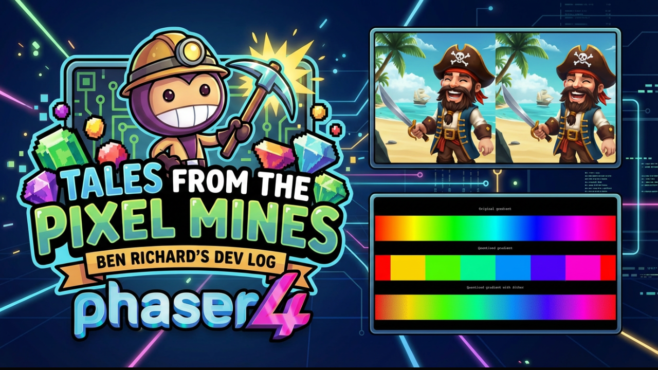
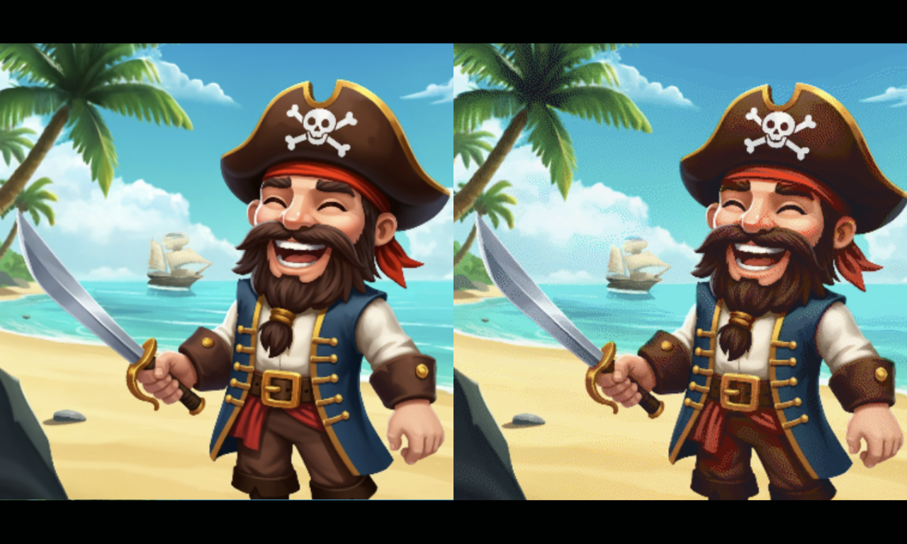
Here's an example of dithering in action. The left version is the original; the right version has a hugely reduced palette, with just 5 colors in the sky. Error diffused dithering smooths out these losses, and makes the image far more pleasing than a bandy mess.
Unfortunately, error diffusion doesn't work on the GPU, where pixels are computed in parallel. What do we do?
Well, as YouTuber Acerola recently publicized, some years back a team of Activision engineers figured out a nice solution. It's called Interleaved Gradient Noise. There are other solutions, like Bayer matrices, but IGN is nice and smooth. So I added it to Gradient. Combined with the Standard Derivatives extension, which allows a fragment to share variables with its neighbors somehow, we can see how fast the gradient is shifting, and dither it an appropriate amount.
Here's an example of IGN dithering in action. (This example uses the Quantize filter - see below - to make the effect more visible.) With just 8 colors, we can replicate a decent facsimile of a rainbow! There are some obvious limitations, but again: just 8 colors.
Now, if you're viewing this image with any kind of scaling, it may look more smooth or perhaps more textured than I intended. This is a limitation of dithering: it only works at the target resolution. Once it's resized, the advantage is lost. Further, many gradients just don't need dithering. So dithering is available as an opt-in config option.
Quantize Filter
You might notice that the Phaser 3 Gradient had an option for "steps". What happened to that?
Well, this is an example of quantization: locking values to a limited set of steps. But gradients aren't the only things that can be quantized. Why not allow it to be used for everything? So I made a Quantize filter.
Quantize is pretty straightforward: you set the step count as a tuple (e.g. [ 8, 8, 8, 8 ]), and a color mode which determines what that tuple means (either RGBA or HSVA). It drops the color count accordingly.
Now, if you do this naively, you'll almost certainly get horrible color banding. So Quantize supports dithering too.
This is a great way to emulate old display types which didn't have many colors. It probably won't match any single real-world hardware type precisely, but it's a good place to start.
There are many possible options for quantization. We picked the two that are most easy to understand. It's also possible to optimize for perceptual qualities, such as prioritizing greens; or even use a fixed palette. These would need to be implemented specially.
GradientMap Filter
The GradientMap filter is an alternative approach to color management. It takes the value/brightness of the image as input, and maps it to a ColorRamp. (Look, it's ColorRamp being used outside a Gradient!)
This can be used for all sorts of effects, but one such is palette replacement. By carefully creating a ramp where the bands are each a solid color, and creating images with brightness levels that match those bands, you can recolor the image to whatever palette you wish.
The main limitation is the number of colors. A grayscale image only has 255 possible brightness levels. You might be able to squeeze out more levels by varying the channels, but that's pretty complicated, especially when you're trying to create art. Still, for an old-school sprite style, 256 colors is often plenty!
Wrapping Up
That's all for now. Gradients and the related filters are more powerful than ever in Phaser 4. We hope you find clever ways to use them in your games!
Ben Richards, Senior WebGL Developer, Phaser Studios Inc